ECCE database – user manual

2.1 Cluster Fields

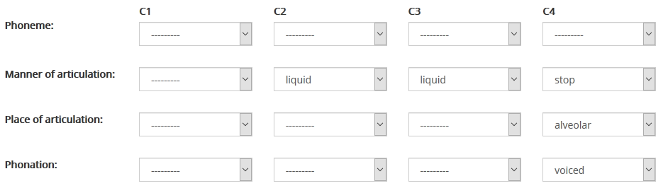
These fields represent the core of ECCE database. They make it possible to search for coda clusters in a variety of different ways. Basically, the database represents clusters as sequences of segments. The maximal length of clusters in our data is four, so the ECCE database search mask contains four columns of search fields, one column for each segment. Column 4 represents the word final segment in a cluster, column 3 the penultimate one, and so on. Each column contains four rows, in which the properties of cluster constituents are represented in four different ways. The first row represents segments as phonemes in IPA notation. The second row specifies their manner of articulation, the third one their place of articulation, and the final one their phonation type (i.e voiced or voiceless). All of the columns may be used in searches for cluster types at different levels of abstraction.

Figure 1 below shows a way of searching for words ending in /rld/ clusters (e.g. world) by looking for sequences of two liquids and a voiced alveolar stop.

(1)

The same clusters would also be returned if one were to search for the final sequence /r/ /l/ /d/, as in figure 2:

(2)

In fact, search fields can be used in any combination. For instance, tokens of world will also be found if one searches for clusters consisting of two liquids followed by /d/, for example, or for clusters consisting of /r/, a liquid, and a final alveolar stop, or for other appropriate combinations. Thus, ECCE makes it possible to search for clusters at various levels of phonological abstraction, and facilitates the investigation of developments that might reflect the impact of markedness constraints on the evolutionary stability of coda clusters. For instance, sonorant-stop clusters (as in old or went) count as less marked than stop-stop clusters (as in act or lagged), and their diachronic stability might reflect this. But this is just an example. The number of phonological hypotheses to test is large.

2.2 The MPT status field

This is the second most important search field in ECCE. It indicates whether clusters are morphotactically compositional or not, and if they are in what way and to what degree. In this field the following categories are distinguished:

1. Morpheme-internal clusters that are licenced by lexical phonotactics, such as /nd/ in wind, or /lp/ in help. They receive the label L.
2. Clusters that come about through and regular inflectional processes, and that span a transparent boundary between stem and suffix, such as /lp+d/ in helped, or /g+z/ in eggs. They receive the label I.
3. Clusters that reflect inflectional processes, but not transparently so. They can count as (partly) lexicalised and receive the label LI.
4. Clusters that come about through derivation, and that span a transparent boundary between stem and suffix, such as /n+θ/ in tenth, or /n+t/ in complaint. g+z/ in eggs. They receive the label D.
5. Clusters that reflect derivational processes, but not transparently so, for instance /l+θ/ in filth or /p+t/ in concept. They can count as (partly) lexicalised and receive the label LD.
6. Clusters within transparent inflectional suffixes, such as the /st/ in goest ‘go’ 2SG, or the /nd/ in lovand ‘loving’ are labelled IS.
7. Word final clusters reflecting inflectional suffixes that have merged with their stems and/or are no longer transparent, such as the /st/ in worst or first are considered lexicalised and labelled LIS.
8. Clusters within transparent derivational suffixes, such as the /nt/ in judgement are labelled DS.
9. Word final clusters reflecting derivational suffixes that have merged with their stems and/or are no longer transparent, such as the /nt/ in parliament are considered lexicalised and labelled LDS.

The possibility of distinguishing, and searching separately, for clusters of different morphotactic categories makes it possible to investigate whether differences in this respect affect the historical stability of clusters. Various theories of morphonology or morphonotactics imply that they should.

2.3 Period fields

Two fields, one representing a starting point and the other an end point, make it possible to limit searches to subsections of the observation period. This allows one to compare coda cluster frequencies and distributions at different historical stages and to identify changes in them.

2.4 The POS field

This field makes it possible to limit searches to specific parts of speech. Labels have been taken over from the Penn Helsinki Parsed corpora, and can be looked up at https://www.ling.upenn.edu/hist-corpora/annotation/index.html. This makes it possible to investigate the distribution of coda clusters among different word classes, and to identify possible correlations and changes in them.

3.1 Basic options: Spelling category

In this field it is possible to specify the structure of clusters in terms of spelling types. ‘C’ stands for consonant graphemes, and ‘E’ for vowel graphs representing likely schwas. Additionally, the symbol ‘_V’ identifies sequences that occur before words beginning with vowel graphs. For example, the filter ‘CCCE_V’ will return tokens like worlde, but only those that are followed by vowels in the text, as in the phrase worlde of sinners.

3.2 Lexicon related search options: Lemma

This section of filters makes it possible to search for word form lemmas. We have found it to be only mildly useful for the main purposes of the database. In order to use it, one needs to be familiar with the specific lemmatization conventions of ECCE (see below → word lemma). If one is, however, this fields allows one to search for spelling variants of specific word types.

3.3 Morphology related search options: Morphonotactic status

This field allows global searches for ‘unambiguously morphonotactic clusters’ (I and D), unambiguously morpheme internal, or ‘lexical’ ones (L, IS and DS), and ‘weakly morphonotactic’ ones (LI, LD, LIS, and LDS).

3.4 Phonology related search options: Right phonological context

Here one can look for clusters that occur before specific consonants in onset of the next word.

3.5 Phonotactics related search options

3.5.1 Cluster size

This field provides a quick way of searching for clusters of different sizes, i.e. for clusters of two, three or four segments.

3.5.2 SSP fulfilled

This field searches for clusters that do or do not fulfil the sonority sequencing principle (Sonority falls towards the end of a cluster, as in /rnd/ as in burned, but not in /pts/ as in adopts).

3.5.3 NAD VC, NAD C1C2, NAD C2C3, and NAD preferred

These fields search for clusters with specific ‘net auditory distances’ (NAD) between their segments. For the concept and how it is measured see http://wa.amu.edu.pl/nadcalc/.

3.6 Text related search options

These allow searches to be restricted to texts of specific genres, specific dialectal regions, or to specific texts. Text identifiers and categorisations are those employed in the Penn Helsinki Parsed Corpora (https://www.ling.upenn.edu/hist-corpora).

4.1 Token list

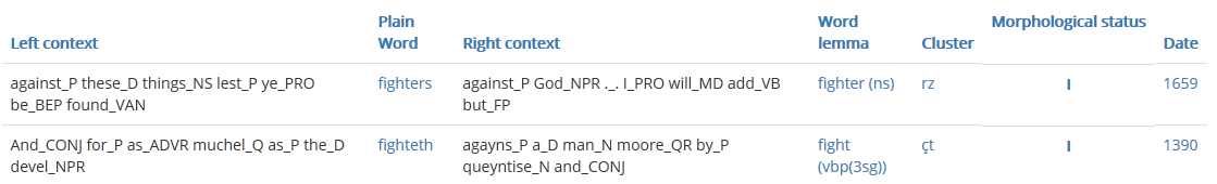
By default the token list will show the following fields:

4.1.1 Plain word

Contains tokens as retrieved from the corpora. The only visible difference is that – for technical reasons - the Penn-Helsinki diacritic ‘+’ is replaced by ‘&’, so that thorn <þ> is now represented as ‘&t’, eth <ð> as ‘&d’, ash <æ> as ‘&a’, and yogh <ʒ> as ‘&g>.

4.1.2 Right context, Left context

Reproduce a bit of the contexts as returned in the POS-tagged files of the Penn-Helsinki corpora. Their purpose is to help users recognize word forms. They do not otherwise figure in the analysis. But see → Right Onset.

4.1.3 Word lemma

Contains ‘lemmas’. We defined as word-form types, rather than as lexemes. Different inflectional forms of a word receive separate lemmas. E.g. wepte, wepest, and wepeþ do not all receive the lemma ‘weep’, but ‘weep (vbd)’, ‘weep (vbp (2sg))’, and ‘weep (vbp (3sg))’ respectively. The morphosyntactic tags we used for the purpose are usually taken over from the Penn Helsinki Corpora (http://www.ling.upenn.edu/histcorpora/annotation/index.html), but some information is added, so that the tags in the ECCE lemmas are sometimes more fine grained. For instance, verbal present tense forms are tagged as ‘VBP’ in the corpora, but we have added person and number as well. For instance, abydest ‘abide.2SG’ is tagged ‘VBP’ (verbal present) in the corpus, but gets the lemma ‘abide (vbp(2sg))’ in ECCE, and the lemma of schuldest ‘should.2SG’ is ‘shall (md(pst.2sg))’. Other conventions we adopted were these:

1. Verbs (including modals and auxiliaries) were lemmatized in their base forms, and additional information such as person or tense is added in the tag (as shown above). E.g. tellen ‘to tell’ → tell(vb); habbe&d ‘he has’ → have(VBP(3sg)); chaungid ‘changed’ → change(vbd) etc.
2. Adjectives and adverbs are lemmatized holistically when derived (i.e. not reduced to their bases: i.e. determined (as in his determined resolution) → determined(adj); bicumeliche → becomely(adv) etc. Adjectives that agree in number or case with the noun are tagged accordingly: equals (as in deuyde it in parties equals, ‘divide it into equal parts’) → equal (adj(pl)).
3. Common and proper nouns are lemmatized in the nominative singular, and inflectional suffixes represented as tags: i.e. dea&des ‘death.GEN’ → death(n$); tymes ‘time.PL’ → time(ns), etc.; Derived word forms are lemmatized holistically, however, and not reduced to their bases: i.e. breadth → breadth(n); cursynge → cursing(n);
4. Personal pronouns are lemmatized in their nominative singular forms - its ‘it.GEN’ → it($), s-derivatives of possessives such as yours are lemmatized as if they were genitives, e.g. yours → your (PRO$).

4.1.4 Cluster

Returns the (actual or potential, see introduction) coda cluster of the word form. The analyses reproduced in this filed need to be handled with some care and responsibly. They are approximations. Among other reasons, this is because we had to generalize over a large observation period, during which segments were subject to considerable variation and change. It was impossible to take this into account. For instance, /x/ in fight probably changed quite gradually from a voiceless fricative to a voiced one, then to an approximant or glide and was eventually completely vocalised. In our database, however, all instances of the word are analysed as ending in the cluster /çt/. There are other cases, which experts will surely notice. In future versions of ECCE the graining of our analyses may become more finely grained, but in the present version it has had to remain approximate. So a detailed look at the results is in certainly still order before conclusions are drawn from them.

4.1.5 Morphological status

Returns the identifiers described above (see → MPT status).

4.1.6 Date

Returns the date at which the token was attested. These dates have been taken over from the Penn Helsinki Corpora, except in cases where the date of composition differed from the date of the manuscript. Here we decided to take the mean. Obviously, this is not completely unproblematic, and ECCE users should refer to the Penn Helsinki Corpora if they decide against living with the consequences of our decision. Also in this case, the ECCE results need to be interpreted with due care.

The token list returned by default thus looks as in figure (3):

(3)

4.1.7 Additional result fields

Apart from the fields returned by default, users may select a number of further result fields to be displayed. These can be accessed by clicking the button under ‘Select additional columns’ on the main search page. Some of them have been created for internal use and may not be very useful for practical purposes. Others might be of interest, however.

4.1.7.1 POS

Returns Penn-Helsinki POS tags.

4.1.7.2 Medial suffix and Final suffix

Return suffixes involved in cluster formation (only in relevant cases, of course).

4.1.7.3 Right onset

Returns the initial segment of the word following the cluster

4.1.7.4 Weight

Returns an estimate of the probability that a token was actually realised with a cluster at the time of its attestation. The single variable taken into account for this purpose is an estimate about the progress of schwa loss. This change represented a major factor in the emergence and rise of coda clusters in English. For instance, in word forms such as clymbe (/’kliːmbə/ > /’kliːmb/) ‘climb’ or ende (/’endə/ > /end/) ‘end’ it changed medial clusters into final ones, and in items like famed (/’faːməd/ > /’faːmd/) ‘famed’ or faylled (/failəd/ >/faild/ ) ‘failed’ new final clusters were created out CVC sequences. Schwa loss spread gradually from the beginning of the twelfth to the end of the fifteenth century, and the probability of potential schwa loss inputs to wind up with a final cluster rose accordingly. For our purpose, we modelled schwa loss spread in terms of an s-curve that we calibrated against evidence from verse texts (see Bauman, Prömer and Ritt forthc.). In relevant tokens, our estimate of the probability that a potential cluster was realised as an actual one is therefore a linear function of our estimate of schwa loss progress. – It is of course evident that the weights thereby attributed to tokens cannot be interpreted literally as saying much (or anything) about individual occurrences. They represent statistical measures and make sense only when one interprets them as being about token populations at particular periods rather than commitments about individuals. Therefore, it makes much more sense to consider their impact on the frequency tables that ECCE offers as well (see below): in a population of 1000 tokens with a cluster probability of 0.7 per token, it clearly makes some sense to think that about 700 of them may have surfaced with an actual coda cluster, even if one does not know which the specific ones that did actually were. It is for such statistical purposes that we have introduced probability weightings into the database, and we have made it possible to look at estimates in the token list primarily for purposes of transparency. Even when interpreted statistically as being about populations rather than individual instances, however, our estimates remain, indeed, estimates and should be handled accordingly and with due caution.

Caveat: It needs to be pointed out in this context that schwa loss is the ONLY variable that we have taken into account when estimating cluster probabilities. Crucially, other sound changes such as the vocalisation of /x/ in words like knight, or the deletion of final /b/ and /g/ in climb or thing do not yet figure in our calculations, although they may do so in later versions. This means that our database overestimates cluster frequencies particularly in the later parts of the observation period. Users interested in clusters to which that applies, will for the present have to adjust the results that ECCE returns accordingly.

4.2 Frequency tables

In addition to token lists, ECCE generates frequency lists for any search one formulates. They can be accessed by clicking on the button ‘See frequency tables’ on the main search page, and look as in figure (4).

(4)

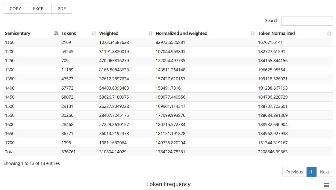
Frequency tables contain the following fields:

4.2.1 Semicentury

Shows the start dates of half centuries in which the returned tokens were attested. I.e. 1350 means 1350-1400 and so on.

4.2.2 Tokens

Shows the absolute number of word form tokens attested in the period that had the potential of ending in a cluster.

4.2.3 Weighted

Shows the absolute number of tokens likely to have been actually realised with clusters taking the progress of schwa loss into account. (Relevant only for statistical significance tests)

4.2.4 Normalized and weighted

Shows the number of tokens per million words that were likely to have been actually realised with clusters taking the progress of schwa loss into account.

4.2.5 Normalised

Shows the number of word form tokens per million words attested in the period that had the potential of ending in a cluster.